All our livelihoods sprout from the top two metres of the earth's crust. Agriculture is a fundamental part of our society... and also of the ecological transition. According to the European Environment Agency, farming accounts for 10% of current greenhouse gas emissions in the EU. And the demand for food is expected to increase by 70% in the coming decades. It is therefore a very relevant sector in the European Green Deal. At the heart of the European Commission's agricultural policies is the CAP - the Common Agricultural Policy. In 2021, CAP accounted for 33% of the total EU budget. A large part of the CAP budget is dedicated to direct payments to farmers:
- they work as a safety net and make farming more profitable;
- they ensure food security in Europe;
- help them produce safe, healthy and affordable food;
- they reward farmers for providing public goods that markets do not normally pay for, such as landscape and environmental protection.
To facilitate the collection and assessment of these payments, Copernicus satellite imagery provides valuable information. In particular, they can allow the European Commission to know the total area that has been cultivated in certain areas. Some time ago we told you about a Deep Learning model that allowed us to identify natural habitats using images from the Copernicus Sentinel-2 satellite. Today we want to talk about a similar approach, but oriented towards agriculture.
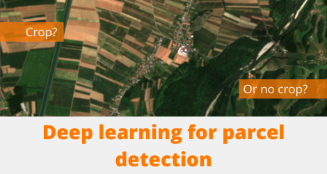
Farm or not farm? That's the question
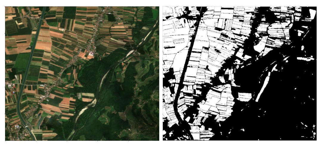
The tool was developed as part of one of the challenges set by AI4EO. The objective of the challenge was to develop a method to map cultivated land using Sentinel satellite imagery, extracting as much information as possible from the image at native 10-metre resolutions. In our case, we have developed a Deep Learning model that differentiates the crop plots in the satellite images and quadruples the original resolution from the original 10 metres to a resolution of 2.5 metres.
Locations
In their challenge, AI4EO identified 100 regions of interest, located in the Republic of Slovenia and neighbouring countries. Each of these regions measures 5x5 km, and contains a lot of information:
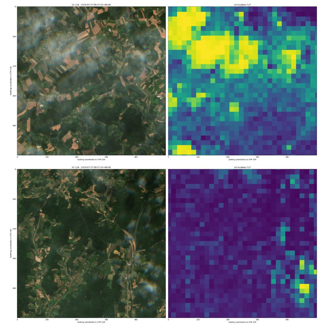
- 12 multispectral bands: from the visible to the shortwave infrared, with a resolution of 10m.
- An information mask to find out if there are clouds in the image. This allows us to discard images that are too cloudy and therefore make it impossible to discern what is on the ground.
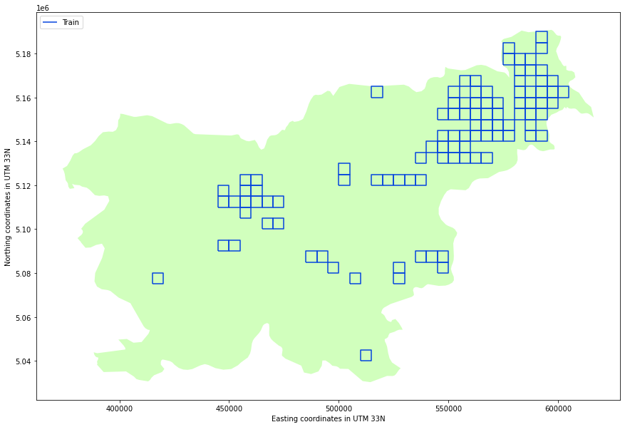
Of these 100 regions, we randomly separate them into 3 types:
- Train: regions that we use to train the models.
- Validation: we reserve these regions to decide the best configuration of the network.
- Test: we use these regions to avoid overfitting the models and to check the generalisability of the models.
How to clean the data
Before training the models, it is important to approach the problem in a constructive way. In our case, we had two main difficulties: discarding "non-useful" data when training the models, and identifying small crop plots. To train the models with useful data, we resorted to cloud masking, which we mentioned earlier. This allows us to discard images where too much information is missing (because clouds cover a large part of the image).
In addition to these spatial filters, in order to select the images where we have more information, we include an additional filter, this time of a temporal nature. The dataset provided by AI4EO covered the period from 1 March to 1 September 2019. In these 6 months, the variability of the field is very high: there are fields that go from being cultivated to being harvested, fields that go fallow... Our model therefore has to be able to extract relationships over time. To account for this variability, we chose only those dates for which we had valid images for all 100 locations. This left us with only 10 days of data: 10 dates where we have a maximum of 20% cloud cover at all locations.
If we look at the images and start to delineate cultivated plots, we have little difficulty identifying the large plots... and our eyes start to suffer when trying to identify the smaller ones. The same thing happens to Deep Learning models. To make it easier for these models to learn to distinguish small plots, we made it so that in the training region, not all plots have the same value (or weight). Uncultivated plots have a weight of 1 for the model. Cultivated plots have a weight between 1 and 2, which follows a skewed normal distribution depending on plot size, as in the picture:
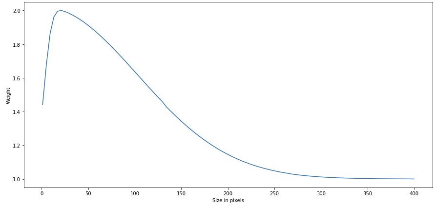
In this way, the model prioritises smaller cultivated plots, since if the plot consists of 5 pixels it will have twice as much weight as if it consists of 400 pixels.
Autoencoder and TFCN: two different Deep Learning models
Once the problem was focused, we decided to train two different models, to see their performance: an autoencoder model and a TFCN (Temporal-Frequential Convolutional Network) model.
Autoencoder model
This model does not use the pre-processed data as is, but a series of vegetation indices, which allow estimating the quantity, quality and development of vegetation. Instead of choosing a single index, we train models for three different indices (NDVI, EVI and RVI) and various combinations. In addition, the increase in resolution of the images is done before the model ingests the data, by linear interpolation.
In the end, what we learned was that NDVI is the most useful index to characterise the crop, and the model did not improve when considering other indices.
TFCN
In this case, the input data to the model is directly the processed data including the time dimension and a series of 3D convolutions are performed. The resolution increase is learned by the model (unlike the autoencoder, where we increase the resolution of the data before giving it to the model).
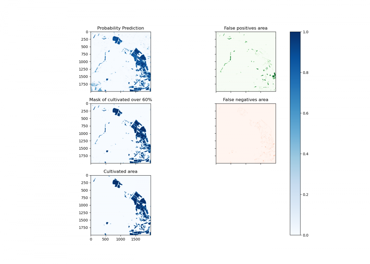
How to interpret the models' results
The two trained models (Autoencoder and TFCN) are probabilistic: instead of saying whether a plot is a field or not, the prediction gives a value between 0 (no cultivation) and 1 (cultivation). Therefore, we have to find a threshold at which to decide whether the plot is a cultivated field or not. The simple option would have been to use 50% as a threshold. However, we decided to refine this approach a little further. Therefore, we resorted to the error function: MCC (Matthews Correlation Coefficient). This is a metric for assessing the quality of binary classifications. The criterion to be followed was that the selected threshold maximises the MCC score. Thus, the chosen threshold is the optimal one to improve the binary classification of crop/non-crop.
Once this was done, there was still room for improvement. Certain water areas systematically gave false positives: they indicated that there was cultivation, when in fact they were water areas. Therefore, we applied an additional water mask, calculated with the ratio of the B2 and B11 bands, based on this work. This approach allowed us to achieve a 0.771 in the MCC function: we ranked seventh in the challenge. By comparison, the winning team achieved an MCC of 0.862. In order to improve these results, we could extend and refine the training dataset.
Although this model applies to agriculture, the approach can bring useful improvements to many other fields. The ecological transition brings with it a lot of questions, many of which have to do with space: How do we organise and use the spaces around us? How much space in the city do we dedicate to green spaces? What about public transport? How do we use the countryside? What are the consequences? For this reason, there are collectives that speak of a second Space Race. In our case, we are proud to be able to contribute to this second conquest of space using tools from the first space race: satellites.