Monitoring agricultural lands, their use and evolution over time; analysing the growth and sustainability of forests and urban areas to plan their management; or developing policies that lay out the agricultural strategies of whole regions. Land management takes care of multiple facets of our environment and is performed through a miriad of institutions: public administrations, regional and national governments and societal platforms. Since their decisions impact whole regions over the course of decades, land management is a sector in continuous renovation, that adjusts measures as information gets updated. Land use or land cover maps are the main tool to do this. Detailed, high-resolution maps that classify locations depending on their type of soil, the vegetation or habitat they present, how that portion of land is used by humans and many other categories. However, developing these maps can be a gruesome process. Traditionally, it involves recurring field work and costly technology—like LiDAR flights— and covered only a portion of the land to be managed. At Predictia, we have developed a Deep Neural Network to generate accurate vegetation maps, using the satellite information provided by Copernicus. In collaboration with the IHCantabria, we have applied this model to develop a vegetation map of the region of Cantabria in Spain.
Want to see the map in action? Explore our interactive Showcase!
The evolution of land use maps: from field trips and flights to satellite imaging
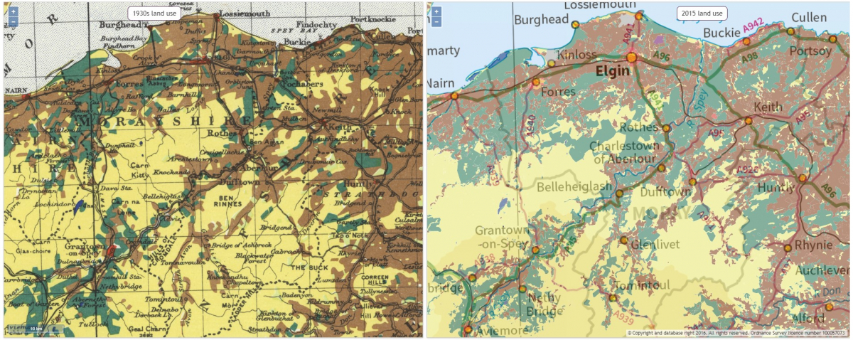
Throughout history, land use maps have not changed that much, but gained in detail and usability. This tool from the National Library of Scotland allows you to compare land use maps from the 1930s with another from 2015.
Soil type maps, vegetation maps, natural resource mapping, urban use… Historically, these land use maps have been a valuable tool, yet very costly to make. Drawing them involves mobilising teams of experts —geographers, geologists, botanists, among others— in costly campaigns. As imaging techniques got better, and automatisation stepped in, the costs went down. Technologies like LiDAR imaging—using laser sensors on a plane to draw altitude maps—helped automating the generation of these maps. However, beside the initial cost of generating the map, keeping them updated is costly. The costs of techniques such as LiDAR flights, together with the costs of mobilising the mapping campaigns, limits the refreshment rate of the maps, usually updated every five years.
The revolution came with the satellite constellations, such as the European Copernicus program. Satellites were constantly observing the Earth, providing an astounding amount of information that can be accessed freely, in many cases. In our case, to develop the vegetation map of Cantabria, we sourced the data from Sentinel 2A and 2B satellites. These two polar-orbiting satellites have a high revisit time: 10 days at the equator with one satellite, and 5 days with 2 satellites (under cloud-free conditions). On mid-latitudes, as is the case of Cantabria, this translates into a 2-3 day revisit time.
Satellites provide a ton of raw data coming from sensors. However, these data still needs to be classified and organised, in order to deliver the actionable tool: the use maps. And here is where Deep learning comes into play.
Using Deep learning to develop a vegetation map
IHCantabria came to us with a clear challenge: developing a vegetation map for Cantabria. The aim was to create a product that would be useful for monitoring the environment and enable public administrators to manage territorial and environmental policies. Such a map had to follow the EUNIS habitat classification: a set of well-defined categories that allows ecologists to identify habitats throughout Europe in a unique way.
To develop this map, we turned to the Sentinel-2 satellites. Specifically to the MSI instrument onboard. Its sensors provide a ton of data, covering 12 different spectral bands that range from the usual three RGB channels that compose the optical imaging, to several infrared bands. Some of these bands are dedicated to measure signals closely linked to vegetation. Like the NDVI signal: a measure of the state of plant health based on how the plant reflects light at certain frequencies (some wavelengths are absorbed and others are reflected).
In the end, we end up with a map of the Cantabria region with very high resolution (10 m). This is an image with over 88 million ground pixels. And for each and everyone of those pixels, we had 12 measurements, coming from the Copernicus remote sensing.
Although we could have developed a vegetation map using just this snapshot of Cantabria, this would have been a pretty standard approach to develop a vegetation map. We wanted to add more value. Since Sentinel satellites revisit the area every 5 days, more or less, we took into account how vegetation changes over time. This provides more accuracy to the final map, while adding another layer of complexity to our model. So, to train our model, IHCantabria facilitated us a homogenised dataset of several snapshots of Cantabria ranging from 2016 to 2019.
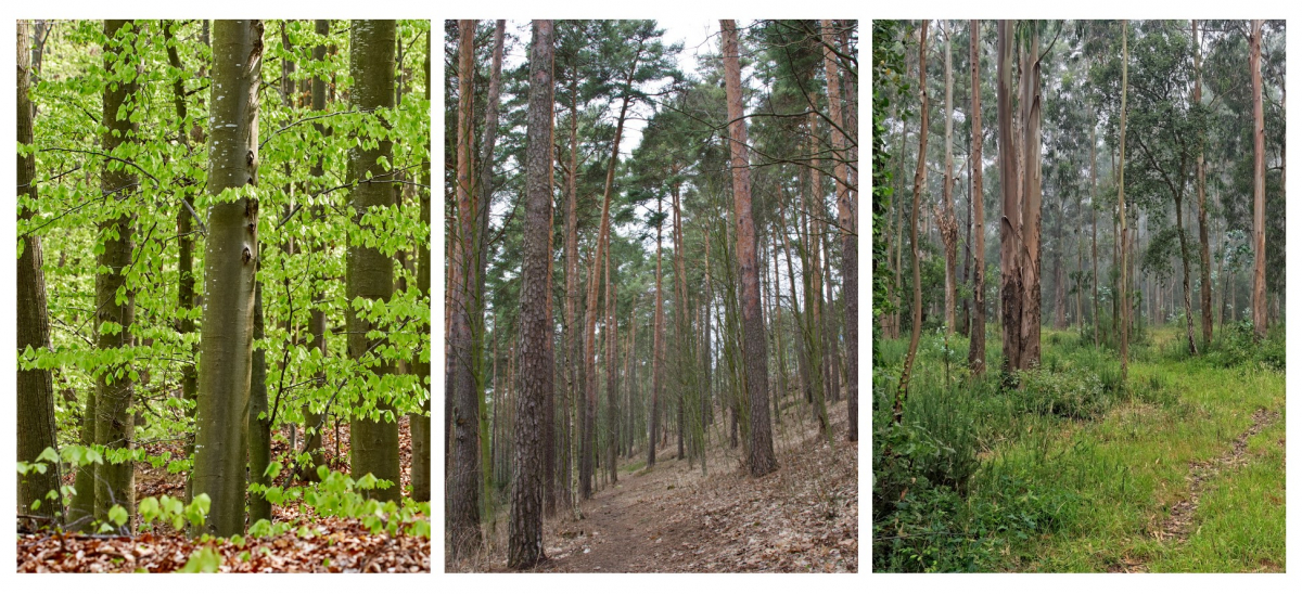
With these highly detailed snapshots, we were ready to train our deep neural network. Since we wanted to model spatial and temporal vegetation variability, we had to handle a high dimensional dataset, so we opted for a Convolutional Neural Network with 3-Dimensional convolutions. There was just a tiny detail: to train our model, we needed a dataset of observed habitats, so the model can classify each pixel from the image. To do that, the botanists at IHCantabria supplied us with a dataset with 26 EUNIS categories. These categories comprehend the most usual vegetation categories in the region, ranging from eucalyptus and native conifer plantations to unbroken pastures and calciphyte bushes.
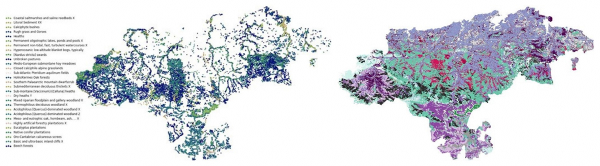
On the left, the dataset with field work data. A portion of these data is used to train the algorithm, while the remaining portion is used to evaluate it. Using that, our model is able to provide the picture on the right: a preliminar map, showing the most probable EUNIS category for each pixel.
For each one of the pixels in the image, our model provides an estimate of the probability that the pixel corresponds to a specific category. To provide the map user with the most useful information possible, we show the information in various ways:
- Providing only the category with the highest score. In this case, the precision of the model is of 59.06%.
- Providing the three categories with the highest score. With this information, the precision rises to an 83.89%.
To develop the model further, we also considered feeding the model with LiDAR imaging provided by IHCantabria. We did it separately, because we didn’t count with LiDAR imaging with the same temporal frequency of the rest of the data, and we wanted to explore the added value of taking the temporal variability into account. LiDAR images, taken by a laser sensor mounted on a plane, provide a height map that is very useful to our Deep Learning model. This data allows to discriminate easily between bushes and trees, just by looking at their height. In this case, thanks to incorporating the LiDAR, the precision rises to a 61.78% when considering only one category, and to an 85.49% with three categories.
Throughout the development, we also managed to optimise the processing time needed to create a vegetation map, cutting down the time from over two weeks to four days. By comparing these with the historic process of developing land use maps, we can see the value that Deep Learning can bring to the table, when joined with the Earth Observation data provided by Copernicus, and working hand in hand with specialised institutions such as IHCantabria.
Explore the interactive map through our Showcase!