Alteration of traditional climate patterns due to climate change effects has made studying adaptation solutions more frequent. Over the past few months we’ve seen catastrophic images of the effects of torrential rainfall across the world from Spain’s Zaragoza to Beijing, where better urban planning, better sewage or a combination of both would have reduce dramatically the impact of water torrents.
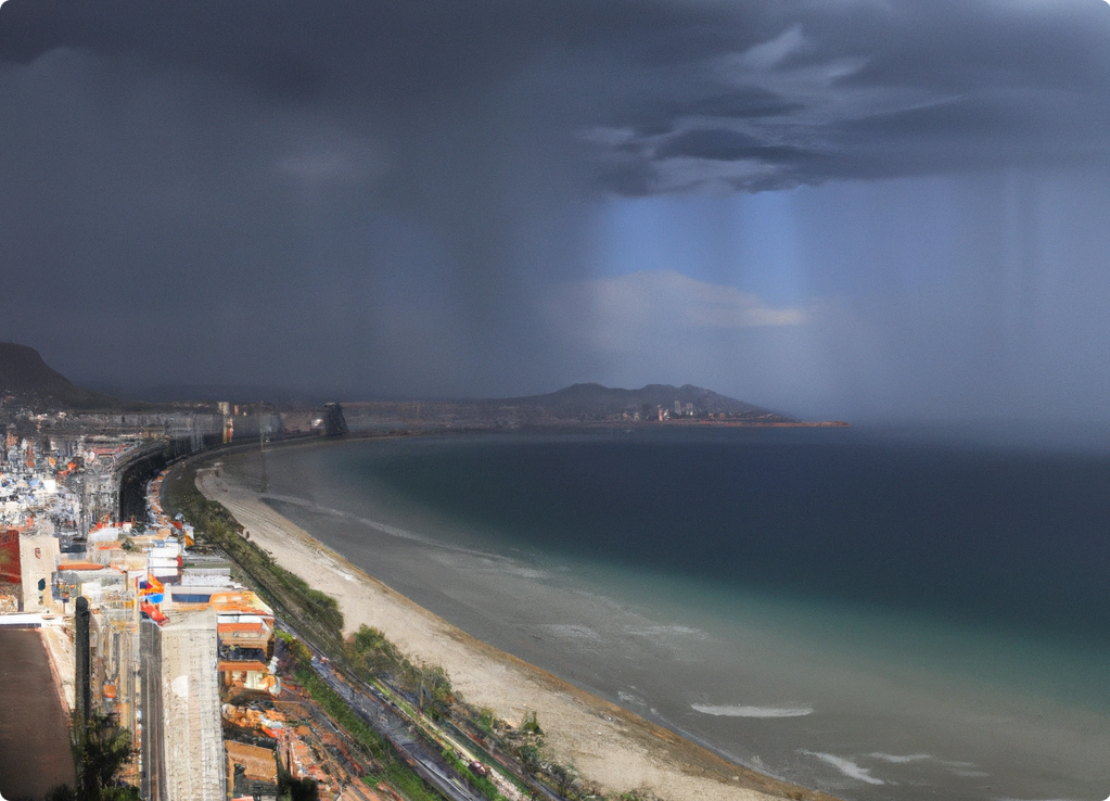
In this post, we’ll be traveling to South Eastern Spain, to the city of Alicante, where rain is progressively shifting its frequency and intensity. Detailed knowledge could help competent authorities and urban planners alike to take better water-management decisions in the city whilst minimising damage when the rains come.
From the early 80s observations show the temperature in the Mediterranean Sea, near which Alicante stands, has risen remarkably.This increase in marine temperature has contributed to a rise in torrentiality of the rains, which are deviating from traditional frequency, torrentiality and seasonality patterns. For example, spring and autumn used to be the seasons were rains concentrated in the region. However, autumn rains have been anticipating to late summer lately. Given this context, it feels necessary to look into these phenomena in order to facilitate data for a successful adaptation strategy.
Climatic projections and bias adjustment
Predictia has participated, together with Aguas de Alicante, in one of the first studies at a national and international level on the application of new mathematical models regarding the urban sewage field. Our contribution has focused on future climate characterisation, for which we used theClimadjust tool to adjust bias of climatic projections coming from a group of climate change models from the Coupled Model Intercomparison Project Phase 6 (CMIP6, 5 simulations) andEURO-CORDEX (51 simulations). Variables taken into account have been precipitation and maximum, minimum and average temperatures.
Precipitation adjustment for the General Circulation Models is done using historical data registered at the official Meteorology State Agency (AEMET) observatory in Ciudad Jardín, in Alicante (38.37ºN, 0.49ºO), for the 1938-2021 period. Temperature projections are based on the ERA5-Landreanalysis as a reference. And taking these series as a base, bias-adjustment techniques are applied (EQM and ISIMIP3) ) to obtain climatic projections in the city. This adjustment has been done for projections in three different greenhouse-gas emission scenarios with daily resolution (CMIP6: SSP1-2.6, SSP2-4.5, SSP5-8.5; and EURO-CORDEX: RCP2.6, RCP4.5, RCP8.5).
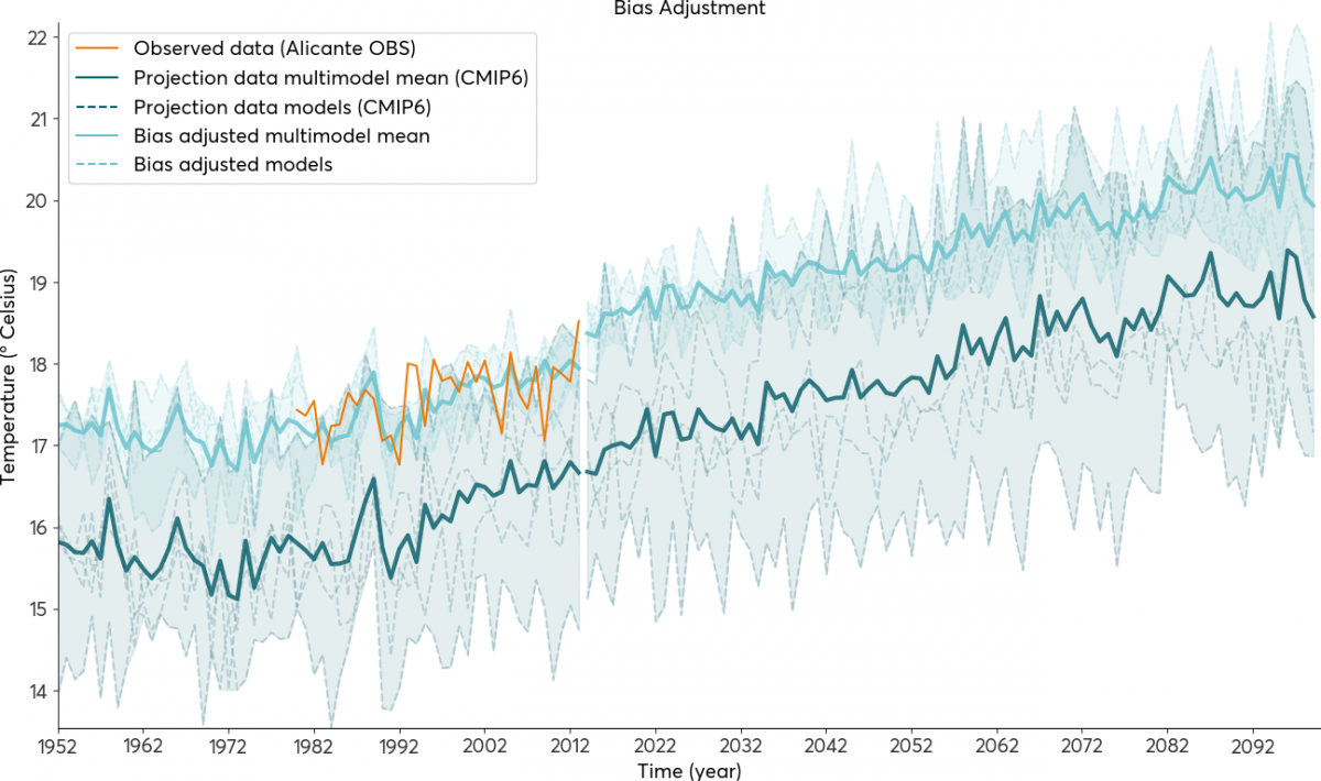
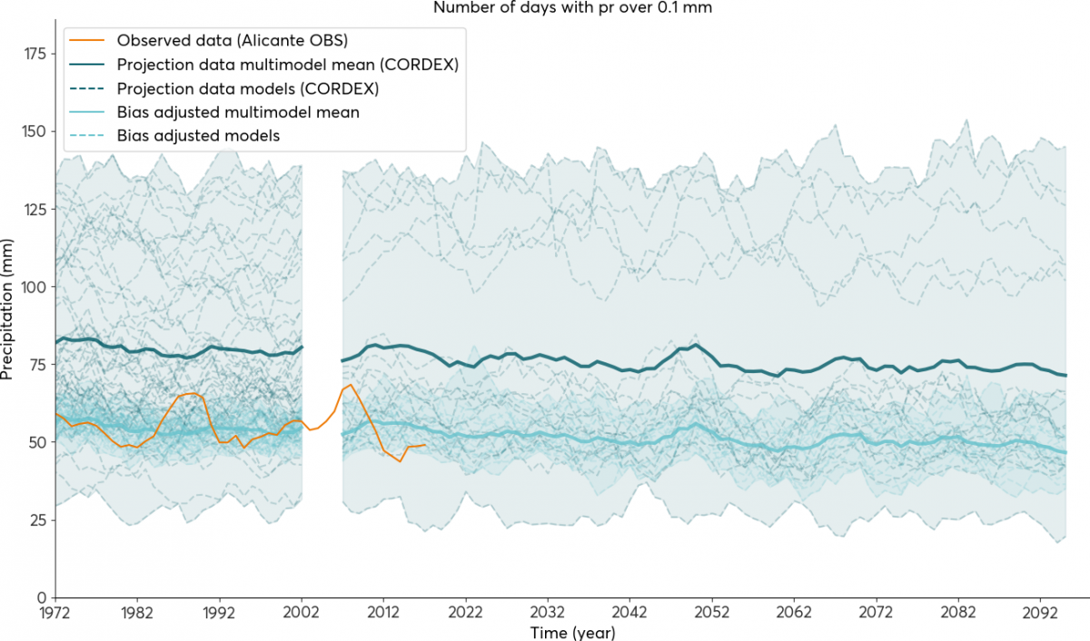
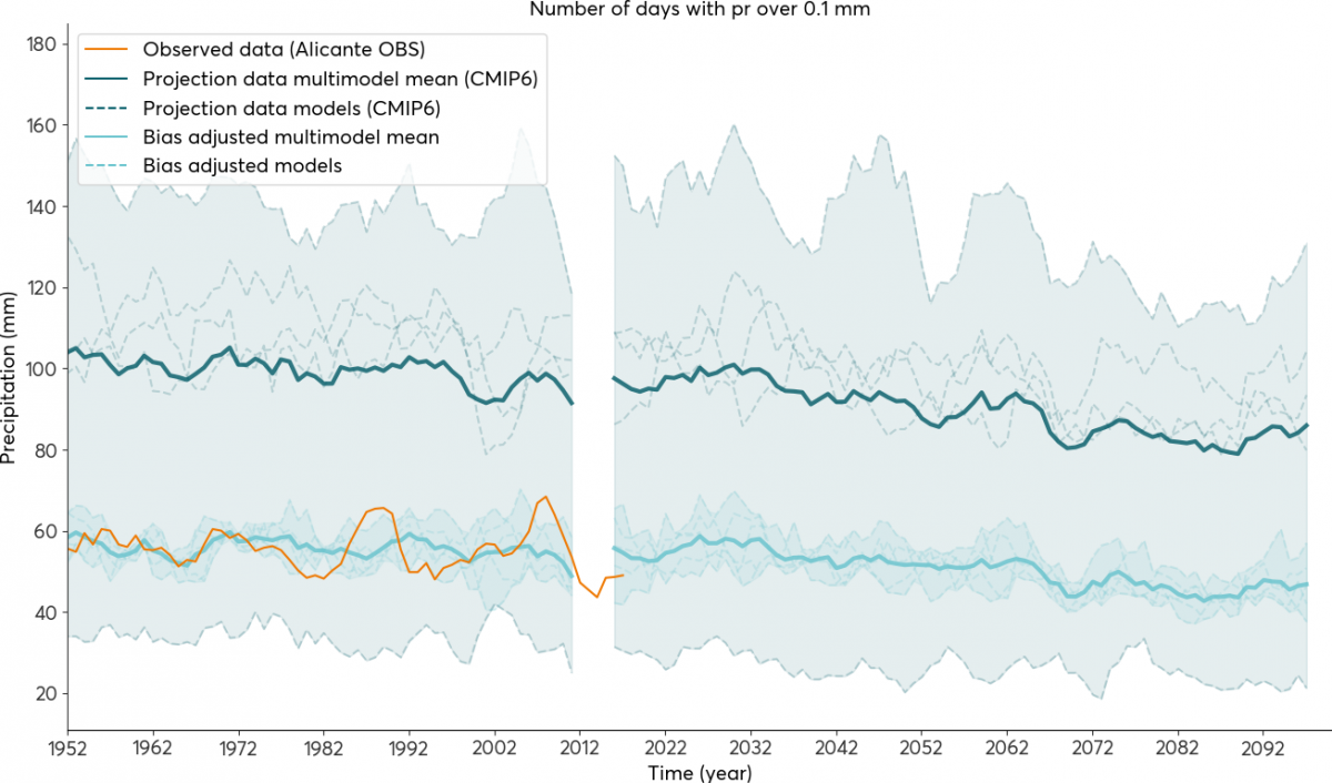
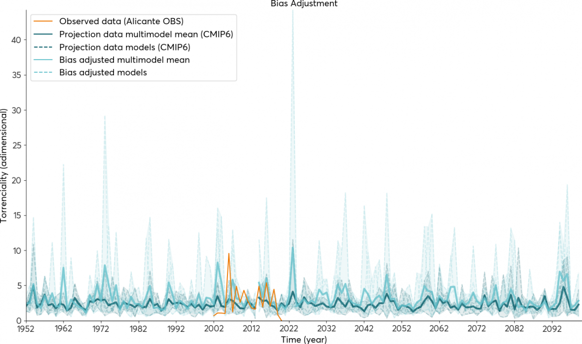
The results obtained from climatic projections with daily resolution show an increase in maximum, minimum and average temperatures, as well as a reduction in the number of rainy days in the city. On figures 1, 2 and 3 you may see that after bias-adjustment techniques are applied, the results are better adjusted to the observations ( light blue and orange lines, respectively), compared to the non-adjusted series (dark blue).
Increase of temporal resolution
Now that climatic projections data are corrected, temporal disaggregation statistical techniques (a cascade model) are used to obtain hourly precipitation series. This is especially interesting for characterization of torrentiality events.
The method used is based on distributing precipitation values in two-interval blocks (see Fig #4). I. e. from 24-hour data, the accumulated precipitation value will be divided in two 12-hour intervals. These will be further subdivided in two 6-hour intervals. And so on until achieving the desired temporal resolution.
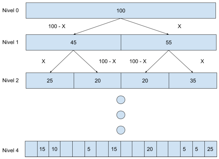
The problem addresses the following question – How are we going to divide precipitation in one of the intervals into two different intervals? There are three possibilities:
- All precipitation is assigned to the first block (100-0).
- X% is assigned to the first block and (100-X)% to the second block.
- All precipitation is assigned to the second block (0-100).
Each of the theoretical distributions can be estimated from observed data. This distribution differentiates between two kinds of rain – above and below a set threshold. These techniques are developed in the open-source Melodist pack.
Intensity-Duration-Frequency (IDF) Curves
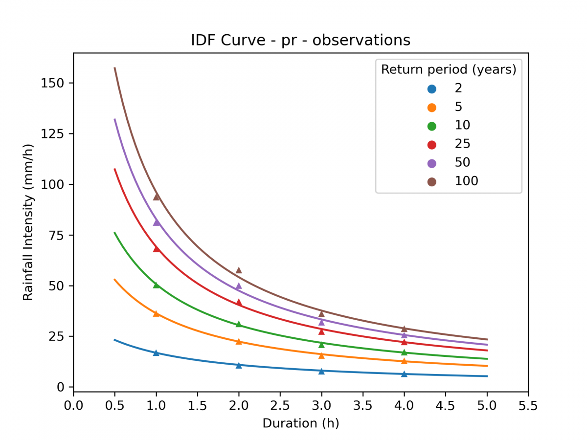
Once the daily precipitation series have been calculated, the IDF curves are obtained from them. Calculating IDF curves is key as water-management infrastructure development is based on these curves, providing extreme values for rain intensity (mm/h) for several durations (minutes to days) with a variable frequency (years).
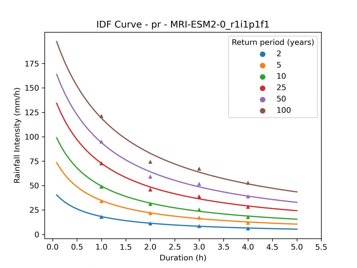
For choosing the best-fitting model or models, the projected IDF curves for the historical scenario 1950-2015 (Fig. #5) are compared to historic AEMET-observed data IDF curves (Fig. #6).
The resulting future climate curves are grouped in climatic periods – near future (2015-2040), mid-term future (2041-2070) and long-term future (2071-2100). These future climate IDF curves are used to calculate the torrentiality rate and the climate change factor for different climate scenarios.
Torrentiality Rate and Climate Change Factor
One of the main goals in this study was to obtain a torrentiality rate that allowed to characterise the frequency and intensity of extreme weaher events. For this, the following methodology was used:
- We calculated the average amount of rain falling on days with values above 1mm.
- We divided the hourly precipitation series by the value of the constant obtained in the previous section.
The objective fo this methodology is identifying hourly intervals when rains falls above the average of a rainy day (see Fig. #7).
For its part, the Climate Change Factor is the percentage variation between the observed intensities and projected ones for future climates, and it’s used for describing the potential development of extreme precipitation due to climate change. If this factor is above 1, the projected intensities will be higher than the ones obtained by observed data, and the change will be bigger the more this departs from 1.
If you’re interested in having a more comprehensive look at this, you may read the following article - Local- scale regionalisation of climate change effects on rainfall pattern: application to Alicante City (Spain), coauthored by our colleagues Antonio Pérez and Mario Santa Cruz and recently published in the prestigious journal Theoretical and Applied Climatology.
Also, should you need tailor-made climate change projections for an specific geographical region, don’t hesitate to reach out to us via predictia@predictia.es or via the Climadjust website.